YouTube trending video data (1) - US
US, Canada & Japan
Background:
This is just for practice and for fun and thus, will only focus on US, Canada and Japan YouTube channels. This will be divided into 3 parts so it won’t be too long.
Dataset
Dataset link: YouTube Trending Video Dataset (updated
daily)
List of YouTube videos that have been on daily trending list from 2020-08-12 to 2022-10-02.
Want to know:
- Top 50 channels and videos that appeared the most on trending
- Top 100 channels and videos with the highest views
- Top 10 channels with the highest revenue sharing
YouTube Channel category
ID - Category name
1 - Film & Animation
2 - Autos
10 -
Music
15 - Pets & Animals
17 - Sports
19 - Travel &
Events
20 - Gaming
21 - Vblogging
22 - Blogs
23 -
Comedy
24 - Entertainment
25 - News & Politics
26 - Howto &
Style
27 - Education
28 - Science & Technology
29 -
Nonprofits & Activism
43 - Shows
Methods
1. Data preparation
1-1. Load libraries
library(tidyr)
library(tidyverse)
## ── Attaching packages ─────────────────────────────────────── tidyverse 1.3.2 ──
## ✔ ggplot2 3.3.6      ✔ dplyr   1.0.10
## ✔ tibble  3.1.8      ✔ stringr 1.4.1
## ✔ readr   2.1.2      ✔ forcats 0.5.2
## ✔ purrr   0.3.4
## ── Conflicts ────────────────────────────────────────── tidyverse_conflicts() ──
## ✖ dplyr::filter() masks stats::filter()
## ✖ dplyr::lag()    masks stats::lag()
library(tibble)
library(dbplyr)
##
## Attaching package: 'dbplyr'
##
## The following objects are masked from 'package:dplyr':
##
##     ident, sql
library(utils)
library(lubridate)
##
## Attaching package: 'lubridate'
##
## The following objects are masked from 'package:base':
##
##     date, intersect, setdiff, union
1-2. Import datasets
US <- read_csv("/Users/Linda/Desktop/RStudio/Kaggle/YouTube/US_youtube_trending_data.csv")
## Warning: One or more parsing issues, see `problems()` for details

## Rows: 185190 Columns: 16
## ── Column specification ────────────────────────────────────────────────────────
## Delimiter: ","
## chr  (7): video_id, title, channelId, channelTitle, tags, thumbnail_link, de...
## dbl  (5): categoryId, view_count, likes, dislikes, comment_count
## lgl  (2): comments_disabled, ratings_disabled
## dttm (2): publishedAt, trending_date
##
## ℹ Use `spec()` to retrieve the full column specification for this data.
## ℹ Specify the column types or set `show_col_types = FALSE` to quiet this message.
2. Data cleaning
2-1. Check for duplicates
sum(duplicated(US)) # 83 duplicate
## [1] 83
2-2. Remove duplicates
# use distinct() to remove duplicates
US <- distinct(US)

# check if it's removed
sum(duplicated(US))
## [1] 0
2.3 - Extract columns we need
We will only look at these columns: title, channel_title, category_id, trending_date, tags, views, likes, dislikes, comment_count
# select columns we need for analysis
# add a "category" column
US_data <- US %>%
  select(title, channelTitle, categoryId, trending_date, tags, view_count, likes, dislikes, comment_count) %>%
  mutate("category" = as.factor(categoryId)) %>%
  mutate(category = recode(category, "1" = "Film", "2" = "Autos", "10" = "Music", "15" = "Pets",
                           "17" = "Sports", "19" = "Travel", "20" = "Gaming", "22" = "Blogs",
                           "23" = "Comedy", "24" = "Entertainment", "25" = "News",
                           "26" = "HowToD", "27" = "Education", "28" = "Science", "29" = "NPO"))

# convert trending date to the date format
US_data$trending_date<- as.Date(US_data$trending_date, format = "%y-%m-%d")

# create a "trending _year" column
US_data <- US_data %>%
  mutate(trending_year = format(trending_date, format = '%Y'))

glimpse(US_data)
## Rows: 185,107
## Columns: 11
## $ title         <chr> "I ASKED HER TO BE MY GIRLFRIEND...", "Apex Legends | St…
## $ channelTitle  <chr> "Brawadis", "Apex Legends", "jacksepticeye", "XXL", "Mr.…
## $ categoryId    <dbl> 22, 20, 24, 10, 26, 24, 26, 27, 24, 10, 22, 22, 20, 10, …
## $ trending_date <date> 2020-08-12, 2020-08-12, 2020-08-12, 2020-08-12, 2020-08…
## $ tags          <chr> "brawadis|prank|basketball|skits|ghost|funny videos|vlog…
## $ view_count    <dbl> 1514614, 2381688, 2038853, 496771, 1123889, 949491, 4704…
## $ likes         <dbl> 156908, 146739, 353787, 23251, 45802, 77487, 47990, 8919…
## $ dislikes      <dbl> 5855, 2794, 2628, 1856, 964, 746, 440, 854, 2158, 4373, …
## $ comment_count <dbl> 35313, 16549, 40221, 7647, 2196, 7506, 4558, 6455, 6613,…
## $ category      <fct> Blogs, Gaming, Entertainment, Music, HowToD, Entertainme…
## $ trending_year <chr> "2020", "2020", "2020", "2020", "2020", "2020", "2020", …
2-4. Check for NAs
We check NA now but not at the beginning because we don’t need to care about NAs in the columns that we don’t use.
sum(is.na(US_data)) # 0 NAs
## [1] 0
No NAs in the columns in our final version of dataset.
3. Data analysis
3-1. All categories
We will start by analyzing all categories and videos to identify general trends from 2020 to the present.
3-1-1. Number times of trending
Which category is the most popular (i.e., appears on trending the most frequently) each year between 2020 and present?
To compare categories and years, we first group the data by trending year and category, and then count the number of times each category appears on trending. We use color to indicate the total number of views for each category.
# no. times on trending of each category
US_channel_trending <- US_data %>%
  group_by(trending_year, category) %>%
  summarise(chtrending_n = n(),
            ch_views_sum = sum(view_count),
            ch_views_avg = ch_views_sum / chtrending_n) %>%
  as.data.frame()
## `summarise()` has grouped output by 'trending_year'. You can override using the
## `.groups` argument.
# Fig 01 - No. times of trending & total views
ggplot(US_channel_trending, aes(y = category, x = chtrending_n, fill = ch_views_sum)) +
  geom_col() +
  facet_grid(. ~trending_year) +
  scale_fill_gradient(low = "light blue", high = "dark blue") +
  theme(axis.text.x = element_text(angle = 90, vjust = 0.5, hjust = 1)) +
  labs(title = 'No. of times on trending of each category (total views)',
       x = '# times on Trending',
       y = 'Category')

The most popular categories for each year between 2020 and present are Entertainment and Gaming videos, as they appeared on trending the most frequently and also had higher total views. It’s worth noting that although music was the third most popular category on trending, it had comparable or higher total views than Entertainment and Gaming, which may be due to people rewatching music videos on YouTube.
# Fig 02 - No. times on trending & average views per trending time
ggplot(US_channel_trending, aes(y = category, x = chtrending_n, fill = ch_views_avg)) +
  geom_col() +
  facet_grid(. ~trending_year) +
  scale_fill_gradient(low = "light blue", high = "dark blue") +
  theme(axis.text.x = element_text(angle = 90, vjust = 0.5, hjust = 1)) +
  labs(title = 'No. times on trending of each category (average views)',
       x = 'No. times on Trending',
       y = 'Category')
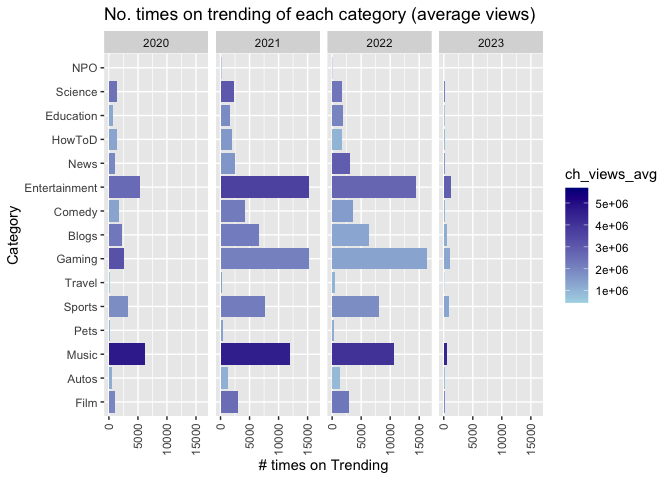
There aren’t many differences between the total views or average views of each category. However, when looking at the average views per trending time, music still has higher or comparable total views to entertainment and gaming.
Next, we identify the channels that have appeared on the trending list more than >200 times. We first group the data by trending year because we want to know what the most popular channels were for each year. Then we group by channel and calculate the number of times each channel appeared on the trending list.
# no. times on trending of each channel
US_channel_trending <- US_data %>%
  group_by(trending_year, channelTitle) %>%
  summarise(chtrending_n = n(),
            ch_views_sum = sum(view_count)) %>%
  as.data.frame()
## `summarise()` has grouped output by 'trending_year'. You can override using the
## `.groups` argument.
# Channels on Trending for >200 times
US_channel_200trending <- US_channel_trending %>%
  arrange(desc(chtrending_n)) %>%
  filter(chtrending_n > 200)

# Fig 03 - Trending times do not correlate with # views
ggplot(US_channel_200trending, aes(y = channelTitle, x = chtrending_n, fill = ch_views_sum)) +
  geom_col() +
  facet_grid(. ~trending_year) +
  scale_fill_gradient(low = "light blue", high = "dark blue") +
  theme(axis.text.x = element_text(angle = 90, vjust = 0.5, hjust = 1)) +
  labs(title = 'Channels on trending >200 times',
       x = 'No. times on trending',
       y = 'YouTube Channels')

It is interesting to note that while Sports is not the most popular category from 2020 to 2022, the NFL and NBA channels are the only channels that have been on trending for more than 400 times each year. This could be due to basketball and football being the two most popular sports in the US.
It is worth mentioning that both of MrBeast’s channels, “MrBeast” and “MrBeast Gaming,” were on trending over 200 times in 2021, but less than 200 times in 2022, experiencing a significant drop in popularity. However, all channels, except for sports channels, experienced a drop in popularity.
To identify videos that have remained on trending for an extended period, we grouped the data by videos and calculated the number of times they appeared on the trending list consecutively for at least a month.
# Videos on Trending for >30 days
USvideo_trending <- US_data %>%
  group_by(title) %>%
  summarise(vtrending_n = n(),
            video_views_sum = sum(view_count),
            category = first(category),
            channelTitle = last(channelTitle)) %>%
  as.data.frame()

US_video_30trending <- USvideo_trending %>%
  arrange(desc(vtrending_n)) %>%
  filter(vtrending_n > 30)

US_video_30trending
##                                                                                            title
## 1                                                                               Starlink Mission
## 2                                              Most Oddly Satisfying Video to watch before sleep
## 3                                                                                    we broke up
## 4                                                            Turn into orbeez - Tutorial #Shorts
## 5                                                               Creative People On Another Level
## 6    Floyd Mayweather vs Logan Paul: Fight goes the distance [Highlights, recap] | CBS Sports HQ
## 7                                        Israeli Iron Dome filmed intercepting rockets from Gaza
## 8       Golden Buzzer: 9-Year-Old Victory Brinker Makes AGT HISTORY! - America's Got Talent 2021
## 9                                                          I Designed Custom Minecraft Bosses...
## 10  India claim stunning series win, end Australia's Gabba streak | Vodafone Test Series 2020-21
## 11 Watch the uncensored moment Will Smith smacks Chris Rock on stage at the Oscars, drops F-bomb
## 12                          The Witch TERRIFIES Simon Cowell to the CORE! | Auditions | BGT 2022
## 13              Highlights: Manchester United 0-5 Liverpool | Salah hat-trick stuns Old Trafford
##    vtrending_n video_views_sum      category         channelTitle
## 1          187       127261126       Science               SpaceX
## 2           50       246738894 Entertainment         SSSniperWolf
## 3           45        65507291 Entertainment    Maddie and Elijah
## 4           36      5640301234 Entertainment               FFUNTV
## 5           35       157562717 Entertainment         SSSniperWolf
## 6           35       554989292        Sports        CBS Sports HQ
## 7           34       789779224          News        The Telegraph
## 8           33       299493829 Entertainment America's Got Talent
## 9           33        41466950     Education        Daniel Krafft
## 10          33      1162813591        Sports       cricket.com.au
## 11          33      3109852918          News        Guardian News
## 12          32       504955736 Entertainment Britain's Got Talent
## 13          31       367867655        Sports         Liverpool FC
Interestingly, SpaceX’s Starlink Mission remained on trending for almost half a year, which is a remarkable achievement.
3-1-2. Highest views
Now, we only select the top 100 videos with highest views.
# rank US videos with top 100 highest views from 2020 to 2022
# total 100 videos
US_channel_top100 <- US_data %>%
  arrange(desc(view_count)) %>%
  slice(1:100)

# rank US videos with top 100 highest views from 2020 to 2022
# total 300 videos = 100 videos per year
US_channel_top100_year <- US_data %>%
  group_by(trending_year) %>%
  arrange(desc(view_count)) %>%
  slice(1:100)

# Category of highest views
US_category_views <- US_channel_top100_year %>%
  group_by(category, trending_year) %>%
  summarise(n_cat_views = n(),
            avg_views = sum(view_count) / n_cat_views) %>%
  as.data.frame()
## `summarise()` has grouped output by 'category'. You can override using the
## `.groups` argument.
# Fig 04 - Top 100 views videos are Music and Entertainment
ggplot(US_category_views, aes(y = category, x = n_cat_views, fill = avg_views)) +
  geom_col() +
  facet_grid(. ~trending_year) +
  scale_fill_gradient(low = "light blue", high = "dark blue") +
  theme(axis.text.x = element_text(angle = 90, vjust = 0.5, hjust = 1)) +
  labs(title = 'Category of videos with top 100 views (2020 - present)',
       x = '# of trending videos in top 100 views',
       y = 'YouTube Category')

The most popular category in 2020 was music, which shifted to entertainment in 2021. In 2022, News and music were the two most popular categories.
# Fig 05 - Channels with videos of top 100 views: Higher views do not correlate with more likes
ggplot(US_channel_top100, aes(y = channelTitle, x = view_count, alpha = likes)) +
  geom_point(color = "blue") +
  facet_grid(. ~trending_year) +
  theme(axis.text.x = element_text(angle = 90, vjust = 0.5, hjust = 1)) +
  labs(title = 'US YouTube Channels with top 100 highest views',
       x = '# of viewss',
       y = 'YouTube Channels')

Black Pink has the highest views.
FFUNTV are mostly shorts!
Big Hit Labels is the former name of HYBE LABELS, which is the company that BTS is belonged to.
# Fig 06 - Top 100 viewed videos: Higher views do not correlate with more likes
ggplot(US_channel_top100, aes(y = title, x = view_count, alpha = likes)) +
  geom_point(color = "blue") +
  theme(axis.text.x = element_text(angle = 90, vjust = 0.5, hjust = 1),
        plot.title = element_text(hjust = -1)) +
  theme_bw(base_family = "NanumGothic") +
  labs(title = 'Top 100 US YouTube videos with highest views',
       x = '# of views',
       y = 'YouTube videos')

4 / 15 videos of highest views are BTS, Black Pink and shorts.
3-1-3. Paid by ad views
We can estimate the revenue sharing for each channel based on the information provided below.
“A good rule of thumb is assuming that only half of your views across the board will be monetized. That said, somewhere around $5-7 per 1,000 views would be the average across all industries.”
Ref: How Much Money Do You Get Per View on YouTube? (2022 Stats)
## Paid by views of each channel
# Fig 07 - All category top 10 of each year
USchannel_pay <- US_data %>%
  group_by(trending_year, channelTitle) %>%
  summarise(view_sum = sum(view_count),
            USD_pay_in_k = (view_sum /1000 * 5)/100 ) %>%
  arrange(desc(USD_pay_in_k)) %>%
  slice(1:10)
## `summarise()` has grouped output by 'trending_year'. You can override using the
## `.groups` argument.
ggplot(USchannel_pay, aes(y = channelTitle, x = USD_pay_in_k, fill = view_sum)) +
  geom_col() +
  facet_grid(. ~trending_year) +
  scale_fill_gradient(low = "light blue", high = "dark blue") +
  theme(axis.text.x = element_text(angle = 90, vjust = 0.5, hjust = 1)) +
  labs(title = 'Amount of top view channel got paid',
       x = 'USD (per 1000 dollars)',
       y = 'Category')

It is estimated that MrBeast has the highest revenue sharing among YouTube channels.
3-2. Channels with excluded categories
Because the channels with high views are typically related to music, movies, sports, and TV shows, we want to exclude those categories to determine which types of channels have higher views.
## Exclude music, films, sports, etc
# list of commercials to be excluded
comm_ch_list <- c("HYBE LABELS", "starshipTV", "Stone Music Entertainment",
                  "NPR Music", "Navrattan Music", "Strange Music Inc",
                  "Zee Music Company", "Desi Music Factory", "MTV",
                  "Paramount Pictures", "Warner Bros. Pictures", "Sony Pictures Entertainment",
                  "Universal Pictures", "Magnolia Pictures & Magnet Releasing",
                  "Orion Pictures", "Marvel Entertainment", "JYP Entertainment", "Big Hit Labels",
                  "Apple", "amazon",  "T-Mobile", "Samsung Mobile USA", "Google")

comm_title_list <- c("Music Video", "Official Video", "Official Music Video", "Official Lyric Video",
                     "Official Audio", "Official MV", "Official Teaser", "Shorts", "shorts",
                     "SHORTS", "Trailer", "TRAILER", "Teaser Video", "TEASER", "M/V", "MV", "Video Oficial")

## Exclude music, films, sports, etc
US_nocomm <- US_data %>%
  filter(categoryId != 2 & categoryId != 17 & categoryId != 25 & categoryId != 43) %>%
  filter(!grepl(paste(comm_title_list, collapse = "|"), title)) %>%
  filter(!grepl(paste(comm_ch_list, collapse = "|"), channelTitle)) %>%
  filter(!grepl('VEVO|Vevo', channelTitle))
3-2-1. Number times of trending of each category
Which category is most popular? (i.e., on trending most often)
# Fig 08 - No. times of trending of each category
US_personal_trending <- US_nocomm %>%
  group_by(category, trending_year) %>%
  summarise(n_personal_trending = n(),
            avg_views = sum(view_count) / n_personal_trending) %>%
  as.data.frame()
## `summarise()` has grouped output by 'category'. You can override using the
## `.groups` argument.
ggplot(US_personal_trending, aes(y = category, x = n_personal_trending, fill = avg_views)) +
  geom_col() +
  facet_grid(. ~trending_year) +
  scale_fill_gradient(low = "light blue", high = "dark blue") +
  theme(axis.text.x = element_text(angle = 90, vjust = 0.5, hjust = 1)) +
  labs(title = 'Top 100 US YouTube videos with highest views',
       subtitle = 'Film, music, TV channels, commercials, shorts are excluded',
       x = 'No. of times on Trending',
       y = 'Category',
       fill = "Average views")

There has been a surge in popularity of personal Gaming and Entertainment content since 2021.
3-2-2. Highest view
Which categories have the most views on YouTube?
# Personal videos of top 100 videos of each year
# total = 300 videos
US_nocomm_top100year_view <- US_nocomm %>%
  group_by(trending_year) %>%
  arrange(desc(view_count)) %>%
  slice(1:100)

# No. days on trending
USnocomm_top100_view_ntrending <- US_nocomm_top100year_view %>%
  group_by(title) %>%
  summarise(channelTitle = first(channelTitle),
            v_ntrending = n(),
            sum_view = sum(view_count)) %>%
  arrange(desc(v_ntrending))

USnocomm_top100_view_ntrending
## # A tibble: 94 × 4
## title chann…¹ v_ntr…² sum_v…³
## <chr> <chr> <int> <dbl>
## 1 I Built Willy Wonka's Chocolate Factory! MrBeast 14 8.15e8
## 2 I Survived 50 Hours In Antarctica MrBeast 11 6.68e8
## 3 Jhoome Jo Pathaan Song | Shah Rukh Khan, Deepika | V… YRF 10 6.11e8
## 4 Galaxy Unpacked January 2021: Official Replay l Sams… Samsung 9 3.04e8
## 5 I Opened A Restaurant That Pays You To Eat At It MrBeast 9 2.63e8
## 6 so long nerds Techno… 9 5.20e8
## 7 1,000 Blind People See For The First Time MrBeast 8 5.93e8
## 8 SHAKIRA || BZRP Music Sessions #53 Bizarr… 8 9.72e8
## 9 100 Kids Vs 100 Adults For $500,000 MrBeast 7 3.69e8
## 10 AMONG US, but with 99 IMPOSTORS The Pi… 7 3.93e8
## # … with 84 more rows, and abbreviated variable names ¹channelTitle,
## # ²v_ntrending, ³sum_view
# Fig 09 - Category of highest views
US_nocomm_top100catyear <- US_nocomm %>%
  group_by(category, trending_year) %>%
  summarise(n_per_cat_views = n(),
            avg_percat_views = sum(view_count) / n_per_cat_views) %>%
  as.data.frame()
## `summarise()` has grouped output by 'category'. You can override using the
## `.groups` argument.
ggplot(US_nocomm_top100catyear, aes(y = category, x = n_per_cat_views, fill = avg_percat_views)) +
  geom_col() +
  facet_grid(. ~trending_year) +
  scale_fill_gradient(low = "light blue", high = "dark blue") +
  theme(axis.text.x = element_text(angle = 90, vjust = 0.5, hjust = 1)) +
  labs(title = 'No. times on trending of categories with top 100 highest views',
       subtitle = 'Film, music, TV channels, commercials, shorts are excluded',
       x = 'No. times on Trending',
       y = 'Category')

Entertainment is the one with highest views from 2020 to 2022.
What are the channels of top 100 videos with highest views?
# Top 100 highest views of total excl. videos
# total = 100 videos
US_nocomm_top100views <- US_nocomm %>%
  arrange(desc(view_count)) %>%
  slice(1:100)

US_nocomm_top100views
## # A tibble: 100 × 11
## title chann…¹ categ…² trending…³ tags view_…⁴ likes disli…⁵ comme…⁶ categ…⁷
## <chr> <chr> <dbl> <date> <chr> <dbl> <dbl> <dbl> <dbl> <fct>
## 1 SHAK… Bizarr… 24 2023-01-20 biza… 1.58e8 8.33e6 0 468245 Entert…
## 2 SHAK… Bizarr… 24 2023-01-19 biza… 1.51e8 8.17e6 0 460932 Entert…
## 3 SHAK… Bizarr… 24 2023-01-18 biza… 1.43e8 7.98e6 0 452536 Entert…
## 4 $456… MrBeast 24 2021-12-02 [Non… 1.37e8 1.09e7 67027 527142 Entert…
## 5 SHAK… Bizarr… 24 2023-01-17 biza… 1.33e8 7.75e6 0 441937 Entert…
## 6 $456… MrBeast 24 2021-12-01 [Non… 1.31e8 1.07e7 62462 516253 Entert…
## 7 SHAK… Bizarr… 24 2023-01-16 biza… 1.23e8 7.45e6 0 427387 Entert…
## 8 $456… MrBeast 24 2021-11-30 [Non… 1.22e8 1.03e7 56591 501543 Entert…
## 9 $456… MrBeast 24 2021-11-29 [Non… 1.11e8 9.69e6 49633 480744 Entert…
## 10 SHAK… Bizarr… 24 2023-01-15 biza… 1.10e8 7.03e6 0 410399 Entert…
## # … with 90 more rows, 1 more variable: trending_year <chr>, and abbreviated
## # variable names ¹channelTitle, ²categoryId, ³trending_date, ⁴view_count,
## # ⁵dislikes, ⁶comment_count, ⁷category
# Fig 10 - Channels of top 100 views videos
# exclude shorts & commercials
ggplot(US_nocomm_top100views, aes(y = channelTitle, x = view_count, alpha = likes, color = trending_year)) +
  geom_point() +
  facet_grid(.~trending_year) +
  theme(axis.text.x = element_text(angle = 90, vjust = 0.5, hjust = 1)) +
  labs(title = 'Top 100 US YouTube channels with highest views',
       subtitle = 'Film, music, TV channels, autos are excluded',
       x = '# of views',
       y = 'YouTube channels')
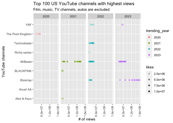
In 2021, MrBeast had the highest views on YouTube. However, in 2023, a new channel has gained popularity - Bizarrap, which is a personal channel of an Argentine DJ and record producer.
What are the vidoes with highest views?
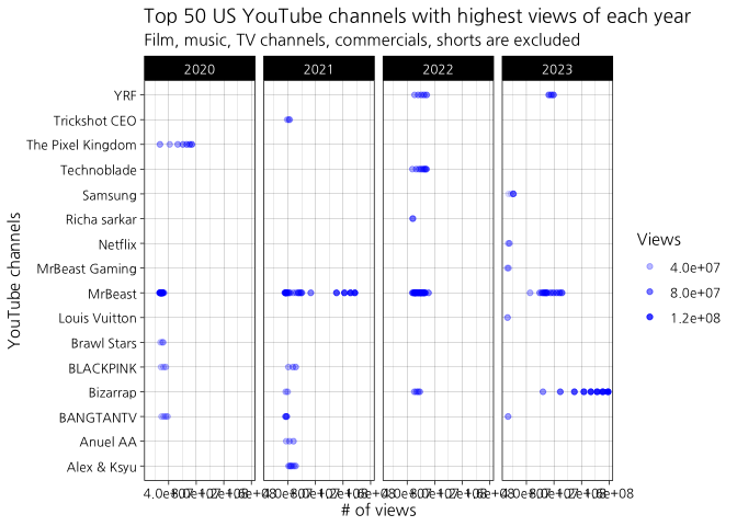
# Fig 11 -  Videos of top 50 highest views (separated by year)
# exclude shorts & commercials
US_top50_view_year <- US_nocomm %>%
  group_by(trending_year) %>%
  arrange(desc(view_count)) %>%
  slice(1:50)

ggplot(US_top50_view_year, aes(y = channelTitle, x = view_count, alpha = view_count)) +
  geom_point(color = "blue") +
  facet_grid(. ~trending_year) +
  theme(axis.text.x = element_text(angle = 90, vjust = 0.5, hjust = 1)) +
  theme_linedraw(base_family = "NanumGothic") +
  labs(title = 'Top 50 US YouTube channels with highest views of each year',
       subtitle = 'Film, music, TV channels, commercials, shorts are excluded',
       x = '# of views',
       y = 'YouTube channels',
       alpha = "Views")
3-2-3. Paid by ad views
Which channels have highest revenue sharing?
US_personal_paytop20 <- US_nocomm %>%
  group_by(trending_year, channelTitle) %>%
  summarise(view_sum = sum(view_count),
            USD_pay_in_k = (view_sum /1000 * 5)/100 ) %>%
  arrange(desc(USD_pay_in_k)) %>%
  slice(1:10)
## `summarise()` has grouped output by 'trending_year'. You can override using the
## `.groups` argument.
# Fig 12 Channels paid - excludes coommercials
ggplot(US_personal_paytop20, aes(y = channelTitle, x = USD_pay_in_k, fill = view_sum)) +
  geom_col() +
  facet_grid(. ~trending_year) +
  scale_fill_gradient(low = "light blue", high = "dark blue") +
  theme(axis.text.x = element_text(angle = 90, vjust = 0.5, hjust = 1)) +
  labs(title = 'US YouTube channels earned (per 1000 views)',
       subtitle = 'Film, music, TV channels, commercials, shorts are excluded',
       x = 'USD (per 1000 dollars)',
       y = 'Category',
       fill = "Views")
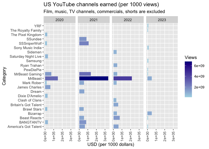
MrBeast is the one have highest revenue sharing since 2020. Other than that, top 10 highest revenue sharing varies for each year.